Gnuplot 5: the Jupyter version

What is it?

In addition to the PDF versions of Gnuplot 5, we offer most of its chapters in the form of Jupyter notebooks. This is a technology that allows you to run programs in many languages, including gnuplot, directly in a web browser, without installing any software. You will see the output of your scripts, including graphics, right on the page. You can save the state of your notebook at any time, or export it as a static document in HTML, PDF, LaTeX, or other formats. This turns Gnuplot 5 into a live, interactive book. It has exactly the same content as the PDF version, except that chapters with no interactive content, such as Chapter 0 on installation, and Chapter 9 on LaTeX, are omitted. We also had to leave out Chapter 10 on arranging multiple graphs, as this does not work in the notebook interface.

Two ways to use it

You can download a zipfile containing all the chapters in Jupyter notebook form from the same place where you download the book and supplementary materials. In order for you to use these downloaded chapters, you will need to have installed Python, Jupyter, and the gnuplot Jupyter kernel.

The other way is to use our gnupyter (gnuplot + Jupyter) service. For this, you will need nothing except a web browser and an internet connection. When you log in to this service, you will get your own space with the latest copies of all the interactive chapters. You can run the scripts from the book to produce graphs, alter the scripts, create new scripts, save different versions of the notebook in your space, etc. You can even switch to the Python kernel if you want to use the notebook for some Python programming. When you come back later, your saved notebooks will still be in your personal space. All the details are below.

Sign up

In your web browser, navigate to https://gnupyter.alogus.com. After the page loads, you should see a login box. You can enter any user name; the password is not used.

If this is your first time logging in to gnupyter, a new notebook will open for you with no content. After a few seconds (or sometimes closer to a minute) you’ll see a collection of chapter notebooks, comprising the interactive version of the book. These are your own copies, that you can modify as you wish. If you save your modified versions, they'll be stored under your username. We don’t guarantee that we’ll keep these files forever, as we may run out of space. Therefore, please make your own backup copies of anything important.

This all means that anyone logging in to the system with your username can see and modify your files. You should treat your username as a password, and keep it secret if you want to protect these files. However, note that your username is stored as plaintext in our system: it’s not encrypted, as a proper password would be. Your notebooks are also not encrypted. Therefore, do not store any sensitive information in your notebooks.

Your dashboard

After logging in, this dashboard should appear after a few seconds. This will have an overview of all your notebooks, and let you do various things to them. At first, there will be nothing there, as shown. After a few seconds, the system will have finished copying the book chapters into your space, and the window should refresh to show you the files. If it doesn’t, you can refresh your browser.

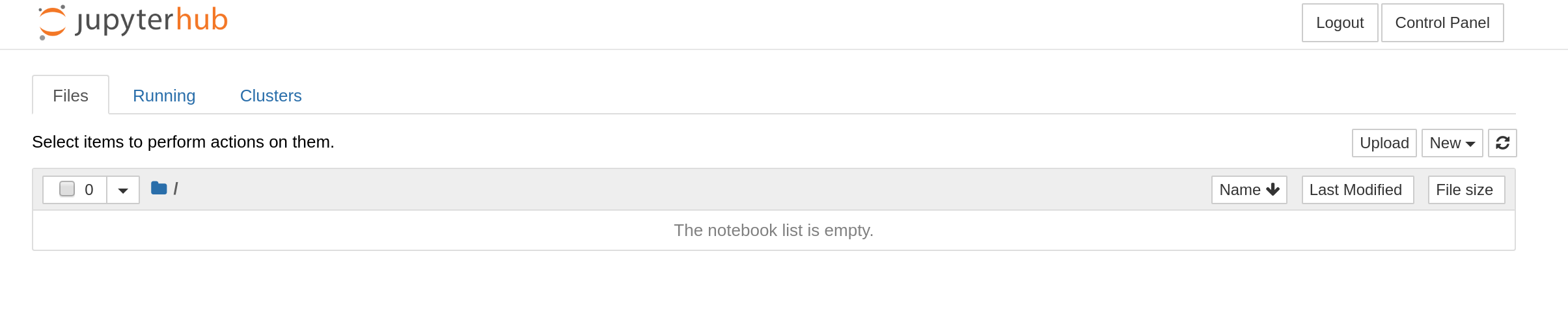
You will see some other files in your dashboard, too: the data files used by the various scripts in the book.

Opening and using a chapter

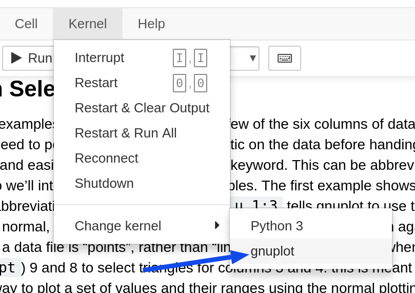
Click on any of the chapters to open it. It will open in a new tab, and takes a few seconds. Jupyter notebooks consist of a series of cells, containing either code or Markdown, for formatted text. All of the scripts in the book have been put in code cells, and all of the text is is Markdown cells. If you put your cursor in any of the code cells and hit shift-enter, or click the “‣Run” button at the top, it will run and you will see the output below the cell. But: you may have to tell the system how to run the cell. It can handle gnuplot and Python code; the first time you open a chapter, you need to tell it to use gnuplot. If you get a syntax error from what looks like normal gnuplot, this is probably the reason. Just choose the gnuplot kernel in the menu at the top.

You can freely modify script cells, insert new cells (using the “+” button at the top), or delete or reorder cells. If you want to save your changes, you will need to select “save as” from the file menu and give your new notebook a name. This is because the chapters supplied to you at the start are read only, so that you will always have pristine book chapters to refer to. After you save a personal version, we’ll keep it for you, so next time you log in you can open it and continue your work.

The formatted text blocks are another type of cell called a “Markdown cell”. You can edit these by double-clicking in them, and return to the rendered form by “running” the cell.

You can also make new notebooks for Python or gnuplot using the file menu; we’ll save these for you, too. You can save and checkpoint notebooks at will, but the system autosaves frequently.

The dashboard, that initial screen from which you opened the chapter file, will always contain a list of all your notebooks. If you accidentally close that tab, you can get it back by selecting open from the file menu.

You can have more than one notebook running at a time. For example, you could have two notebooks running two different languages. Some people use one notebook for exploring, and a second one to copy things into to make a report (see the section on adding descriptive text in this tutorial).

It’s a good idea to shut down of all of them, and log out of your dashboard, when you are done, so you don’t leave anything running. But if you forget, it’s not a disaster.

Tips

Limitations of the notebooks

Your browser needs to have JavaScript enabled. Trying to use a phone for this is probably not going to be a great experience, but it should work.

Along with all the advantages in interactivity come a few limitations. In the book we highlight, with boldface, new occurrences of commands in scripts, to make it easier for the reader to find them. This is not possible in the executable scripts in the notebook. We have left references to the existence of highlighting in the text, however.

The typography in the text cells in the notebooks is not of the same quality as in the PDF version of the book. This is inevitable, as it is HTML rendered by your browser. For example, figures are not wrapped identically, and, in one or two cases, figures in the text do not appear in the notebook versions.

Hyperlinks to documents elsewhere on the web work just as well in the notebooks as they do in the PDF version. However, links to places within the book do not work in notebooks.

There is no table of contents nor index for the notebook version.

A Jupyter notebook maintains a global state. Normally this would mean that a setting in one executed script will still be in effect when you execute other scripts. In the book, each script was run on a freshly started gnuplot instance. In order to get results from the notebook scripts that match the book, a reset command is automatically run at the top of each cell. So if you want to change any settings, just make sure that you put them in any script cell where you want them to be in effect.

Weird errors?

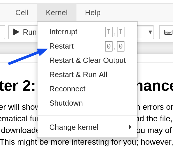
If you are getting weird errors from correct commands (such as a complaint about an “undefined variable” x when issuing a correct comment such as plot sin(x)) and you are sure that you are running the gnuplot kernel (instead of Python), you need to restart the kernel:

Terminals, image sizes, etc.

The default graph size in the notebook is set to be the same as used in the book, so the plot output should look the same.

If you need a different aspect ratio or, perhaps, a higher-resolution image for publication, simply add a terminal setting to the beginning of the script, for example

set term pngcairo size 1200, 600

Images are embedded into the page as data. The most convenient way to save them to your computer is to use your browser’s contextual menu. In this way you can get jpegs or other image formats as well. Note that the images will be displayed resized to fit into the browser window, but they will have the requested pixel dimensions if you save them.

If you want an SVG, you can do the same. The output will be the text of the SVG image, which you can copy.

Other notes

The version of gnuplot backing the notebook is 5.4; it has the help system included, so you can get online gnuplot help, the same as from the gnuplot REPL. Just create a cell and type, for example, help isosurface in the cell, then run it to see gnuplot’s explanation for that command or concept.

Getting help

The author, who also did most of the technical work to put together the gnupyter service, has set up a page where you can ask questions or post comments—about gnupyter, gnuplot, or the book. This is probably the fastest and best way to get assistance.